On Pricing Options with Finite Difference Methods
Introduction
In this notes, finite difference methods for pricing European and American options are considered. We test explicit, implicit and Crank-Nicolson methods to price the European options. For American options, we implement intuitive Bermudan approach and apply the Brennan Schwartz algorithm to prevent the error propagation. Results of simple numerical experiments are shown in the end of notes. This project is implemented using Python objected-oriented programming[code].
Foundations of Finite Difference Methods
In this section, we describe the fundamental ideas of finite difference applied to solve the PDE. This section includes approximation of partial derivatives, general discussion of the grid, and the way of formulating boundary conditions.
The Grid
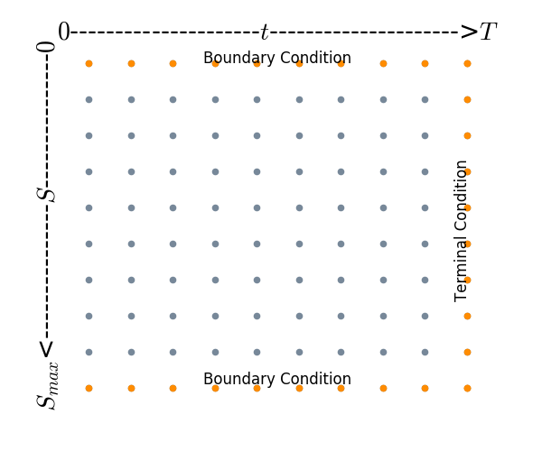
Consider the Black-Scholes equation in the last section, we perform a discretization leading to a two-dimensional grid. To set up a grid, firstly, we should determine the value of $S_{max}$, which is considered as the underlying price unlikely to be reached. Then we discretize the $t$ and $S$ as following,
$$t = 0, \delta t, 2\delta t, …, N\delta t$$
$$S = 0, \delta S, 2\delta S, …, M\delta S$$
$\delta t$ and $\delta S$ are the mesh sized of the discretization of $t$ and $S$. Following figure illustrates part of the entire grid in the $(S, t)$-plane. For each node $(i\delta S, j\delta t)$, we use the grid notation
$$f_{i, j} = f(i\delta S, j\delta t)$$
Theoretical solution $f_{i, j}^{*} $ of Black-Scholes equation is defined on the continuous space. In contrast, the approximation solution $f_{i, j}$ derived from the discretization of the equation is only defined for the nodes. By controlling the parameters $S_{max}, M, N$ , discretization error can be reduced such that $f_{i, j}$ is closer to $f_{i, j}^{*}$ .
Difference Approximation
With the help of Taylor expansion, we can discretize the derivatives in the PDE leading to a recursive formula for $f_{i, j}$. Let us briefly review Taylor expansion and derivatives approximation that derived from it. Assume $f\in C^{(n+1)}$, h is small. For intermediate number $\xi$ between $x$ and $x+h$,
$$f(x+h) = f(x) + hf’(x) + {1\over 2}h^2f’’(x) + … + {h^n\over n!}f^{(n)}(x) + {h^{n+1}\over (n+1)!}f^{(n+1)}(\xi) \tag{1}$$
Replacing terms after $h^2$ with $O(h^2)$ and moving $f’(x)$ to the left-hand side, we have forward difference, which has error order 1
$$f(x+h) = f(x) + hf’(x) + O(h^2) \tag{2}$$
$$\Rightarrow f’(x) = {f(x+h)-f(x)\over h} + O(h) \tag{3}$$
Likewise, we can approximate $f’$ and $f’’$ by backward difference and central difference. Following is a summary of derivatives approximation, expanding at $(i\delta S, j\delta t)$:
| Method | S | t | error order |
|---|---|---|---|
| Forward Difference | ${\partial f\over \partial S} = {f_{i+1,j} - f_{i,j}\over \delta S}$ | ${\partial f\over \partial t} = {f_{i,j+1} - f_{i,j}\over \delta t}$ | 1 |
| Backward Difference | ${\partial f\over \partial S} = {f_{i,j} - f_{i-1,j}\over \delta S}$ | ${\partial f\over \partial t} = {f_{i,j} - f_{i,j-1}\over \delta t}$ | 1 |
| Central Difference | ${\partial f\over \partial S} = {f_{i+1,j} - f_{i-1,j}\over 2\delta S}$ | ${\partial f\over \partial t} = {f_{i,j+1} - f_{i,j-1}\over 2\delta t}$ | 2 |
| Second Difference | ${\partial^2 f\over \partial S^2} = {f_{i+1,j} - 2f_{i,j} + f_{i-1,j}\over \delta S^2}$ | 2 |
Boundary Conditions
Before delving into the finite difference based pricing algorithm, we need to discuss the choice of boundary conditions which is an important issue in the construction of these pricing methods. Well chosen boundary conditions contribute to preventing any errors on the boundaries propagated through the rest of the mesh. There are several ways to specify boundary conditions:
Dirichlet Condition
A Dirichlet boundary condition is a boundary condition which assigns a value to $f$ at boundary. For example, for a call option at $S_{min}=0$ , the option value could be set to zero, since the option is worthless. However, if underlying price reaches to $S_{max}$ at time $t$, the value of option is the discounted value of its expected payoff.For a vanilla call option:
$$f(S_{max}, t) = S_{max}-Ke^{-r(T-t)} \tag{5}$$
$$f(0, t) = 0 \tag{4}$$For a vanilla put option
$$f(0, t) = Ke^{-r(T-t)} \tag{6}$$$$f(S_{max}, t) = 0 \tag{7}$$
Neumann Condition
Neumann condition specifies the partial derivative of the option at the boundary. Discretizing the second derivative at the boundary by central difference gives us a more friendly equation about $f_{i,j}$. In addition, the Neumann condition is inclined to be more accurate for the same boundaries than the Dirichlet condtion, as the second derivatives falls off faster than the price. And Neumann condition is more universal, same for both call and put, and on both ends.
$${\partial^2 f\over \partial S^2}(\delta S, t) = 0 \tag{8}$$$${\partial^2 f\over \partial S^2}((N-1)\delta S, t) = 0 \tag{9}$$
$$\Rightarrow f_{0,j}-2f_{1,j}+f_{2,j} = 0 \tag{10}$$ $$\Rightarrow f_{M-2,j}-2f_{M-1,j}+f_{M,j} = 0 \tag{11}$$
Finite Difference Methods
In this section, we discretize the B-S PDE using explicit method, implicit method and Crank-Nicolson method and construct the matrix form of the recursive formula to price the European options. Graphical illustration of these methods are shown with the grid in the following figure. In the next part, we discuss two pricing algorithms for American option, Bermudan Approximation Method and Brennan Schwartz Algorithm.
Explicit Method
Discretization
Use backward difference approximation for t and central difference for S, expanding at $(i\delta S, j\delta t)$, $${f_{i,j}-f_{i,j-1}\over dt} + ridS{f_{i+1,j}-f_{i-1,j}\over 2dS} + {1\over 2}\sigma^2(idS)^2{f_{i+1,j}-2f_{i,j}+f_{i-1,j}\over (dS)^2} = rf_{i,j} \tag{12}$$ By algebraic rearranging, we end up with the formula we need to implement to price the options, $$\alpha_i f_{i-1,j} + (1-\beta_i)f_{i,j} + \gamma_i f_{i+1,j} = f_{i,j-1} \tag{13}$$$$\alpha_i = {1\over 2}idt(i\sigma^2-r) \tag{14}$$
$$\beta_i = -dt(i^2\sigma^2+r) \tag{15}$$
$$\gamma_i = {1\over 2}idt(i\sigma^2+r) \tag{16}$$
With this recursive formula, the grid and boundary conditions, we are now equipped to solve the B-S equation by the explicit finite difference method.
Matrix Form
Formula (13) can be represented in matrix form:
$$
\begin{bmatrix}
1+\beta_1 & \gamma_1 & 0 & \cdots & 0 \\
\alpha_2 & 1+\beta_2 & \gamma_2 & \cdots & 0 \\
0 & \alpha_3 & 1+\beta_3 & \cdots & 0 \\
\vdots & \vdots & \vdots & \ddots & \gamma_{M-2}\\
0 & 0 & 0 & \alpha_{M-1} & 1+\beta_{M-1} \\
\end{bmatrix}
\begin{bmatrix}
f_{1,j} \\
f_{2,j} \\
f_{3,j} \\
\vdots \\
f_{M-1,j} \\
\end{bmatrix} +
\begin{bmatrix}
\alpha_1 f_{0,j} \\
0 \\
0 \\
\vdots \\
\gamma_{M-1} f_{M,j} \\
\end{bmatrix} =
\begin{bmatrix}
f_{1,j-1} \\
f_{2,j-1} \\
f_{3,j-1} \\
\vdots \\
f_{M-1,j-1} \\
\end{bmatrix}
\tag{17}$$
Substituting the formula of Neumann condition (10) and (11) into $f{0,j}$ and $f{M,j}$, we have
$$ \begin{bmatrix} 2\alpha_1 + 1+\beta_1 & \gamma_1 - \alpha_1 & 0 & \cdots & 0 \\ \alpha_2 & 1+\beta_2 & \gamma_2 & \cdots & 0 \\ 0 & \alpha_3 & 1+\beta_3 & \cdots & 0 \\ \vdots & \vdots & \vdots & \ddots & \gamma_{M-2}\\ 0 & 0 & 0 & \alpha_{M-1} - \gamma_{M-1} & 2\gamma_{M-1} + 1 + \beta_{M-1} \\ \end{bmatrix} \begin{bmatrix} f_{1,j} \\ f_{2,j} \\ f_{3,j} \\ \vdots \\ f_{M-1,j} \\ \end{bmatrix} = \begin{bmatrix} f_{1,j-1} \\ f_{2,j-1} \\ f_{3,j-1} \\ \vdots \\ f_{M-1,j-1} \\ \end{bmatrix} \tag{18}$$ Recall that values of grid are calculated moving backward in time. In hence, we can explicitly solve the $f_{j-1}$. Actually, instead of using the matrix multiplication, we would better calculate $f_{j-1}$ using the recursive formula () directly, which is faster and clear.Implicit Method
Discretization
Use forward difference approximation for t and central difference for S, expanding at $(i\delta S, j\delta t)$,
$${f_{i,j+1}-f_{i,j}\over dt} + ridS{f_{i+1,j}-f_{i-1,j}\over 2dS} + {1\over 2}\sigma^2(idS)^2{f_{i+1,j}-2f_{i,j}+f_{i-1,j}\over (dS)^2} = rf_{i,j} \tag{19}$$
By algebraic rearranging, we end up with the formula we need to implement to price the options,
$$\alpha_i f_{i-1,j} + (1+\beta_i)f_{i,j} + \gamma_i f_{i+1,j} = f_{i,j+1} \tag{20}$$
$$\alpha_i = {1\over 2}idt(r-i\sigma^2) \tag{21}$$
$$\beta_i = dt(r+i^2\sigma^2) \tag{22}$$
$$\gamma_i = -{1\over 2}idt(r+i\sigma^2) \tag{23}$$
With this recursive formula, the grid and boundary conditions, we are now equipped to solve the B-S equation by the implicit finite difference method.
Matrix Form
Matrix form of B-S equation discretized by implicit method has similar form as that of explicit method.
$$
\begin{bmatrix}
2\alpha_1 + 1+\beta_1 & \gamma_1 - \alpha_1 & 0 & \cdots & 0 \\
\alpha_2 & 1+\beta_2 & \gamma_2 & \cdots & 0 \\
0 & \alpha_3 & 1+\beta_3 & \cdots & 0 \\
\vdots & \vdots & \vdots & \ddots & \gamma_{M-2}\\
0 & 0 & 0 & \alpha_{M-1} - \gamma_{M-1} & 2\gamma_{M-1} + 1 + \beta_{M-1} \\
\end{bmatrix}
\begin{bmatrix}
f_{1,j} \\
f_{2,j} \\
f_{3,j} \\
\vdots \\
f_{M-1,j} \\
\end{bmatrix} =
\begin{bmatrix}
f_{1,j+1} \\
f_{2,j+1} \\
f_{3,j+1} \\
\vdots \\
f_{M-1,j+1} \\
\end{bmatrix}
\tag{24}$$
Crank-Nicolson Method
Discretization
Using central difference on both $t$ and $S$, we discretize B-S equation at $(i\delta S, (j+{1\over2})\delta t)$. Specifically, we use the average of first derivative on $(i\delta S, (j+1)\delta t)$ and $(i\delta S, j\delta t)$ to approximate the the first derivative on $(i\delta S, (j+{1\over2})\delta t)$. The second derivative is obtained in the same way. We have,
$${\partial f\over \partial t}(S_i, t_{j+{1\over2}}) = {f_{i,j+1} - f_{i,j}\over \delta t} \tag{25}$$ $${\partial f\over \partial S}(S_i, t_{j+{1\over2}}) = {1\over2}( {\partial f\over \partial S}(S_i, t_{j+1}) + {\partial f\over \partial S}(S_i, t_{j}) ) = ... \tag{26}$$ $${\partial^2 f\over \partial S^2}(S_i, t_{j+{1\over2}}) = {1\over2}({\partial^2 f\over \partial S^2}(S_i, t_{j+1}) + {\partial^2 f\over \partial S^2}(S_i, t_{j})) = ... \tag{27}$$Then we discretize first and second derivatives and plug them into the B-S equation, we have
$$-\alpha_i f_{i-1,j} + (1-\beta_i)f_{i,j} - \gamma_i f_{i+1,j} = \alpha_i f_{i-1,j+1} + (1+\beta_i)f_{i,j+1} + \gamma_i f_{i+1,j+1} \tag{28}$$$$\alpha_i = {1\over4}idt(i\sigma^2-r) \tag{29}$$
$$\beta_i = -{1\over2}dt(i^2\sigma^2+r) \tag{30}$$
$$\gamma_i = {1\over 4}idt(i\sigma^2+r) \tag{31}$$
Matrix Form
Using Neumann boundary conditions, we simplify the matrix equation and end up with following formula,
$$
\begin{bmatrix}
-2\alpha_1 + 1-\beta_1 & -\gamma_1 + \alpha_1 & 0 & \cdots & 0 \\
-\alpha_2 & 1-\beta_2 & -\gamma_2 & \cdots & 0 \\
0 & -\alpha_3 & 1-\beta_3 & \cdots & 0 \\
\vdots & \vdots & \vdots & \ddots & -\gamma_{M-2}\\
0 & 0 & 0 & -\alpha_{M-1}+\gamma_{M-1} & -2\gamma_{M-1}+1- \beta_{M-1} \\
\end{bmatrix}
\begin{bmatrix}
f_{1,j} \\
f_{2,j} \\
f_{3,j} \\
\vdots \\
f_{M-1,j} \\
\end{bmatrix} = \\
\begin{bmatrix}
2\alpha_1 + 1+\beta_1 & \gamma_1 - \alpha_1 & 0 & \cdots & 0 \\
\alpha_2 & 1+\beta_2 & \gamma_2 & \cdots & 0 \\
0 & \alpha_3 & 1+\beta_3 & \cdots & 0 \\
\vdots & \vdots & \vdots & \ddots & \gamma_{M-2}\\
0 & 0 & 0 & \alpha_{M-1} - \gamma_{M-1} & 2\gamma_{M-1} + 1 + \beta_{M-1} \\
\end{bmatrix}
\begin{bmatrix}
f_{1,j+1} \\
f_{2,j+1} \\
f_{3,j+1} \\
\vdots \\
f_{M-1,j+1} \\
\end{bmatrix}
\tag{32}$$
Consistency, Stability and Convergence
When discussing effectiveness of different finite difference methods, we should consider three fundamental properties, which are consistency, stability, and convergence. Before that, we have to notice that though numerical method is good for solving PDE, it also brings the truncation error. Two important sources of error are the truncation error in discretization of stock price and time space.
- stability: A finite difference scheme is said to be stable if the difference between numerical solution and the true solution will not grow unboundedly as $dS$ and $dt$ approach zero. The stability of numerical scheme is achieved if the spectral radius of $A$ less than 1.
- consistency: A finite difference scheme is consistent if the difference between PDE and finite differential equation vanishes as $dS$ and $dt$ approach zero. That is, the truncation error tends to 0 as the mesh get infinitely finer.
- convergence: A finite difference scheme is said to be convergent if solutions derived from a finite difference equation converge point-wise to the true solutions of the original PDE as $dS$ and $dt$ approach zero.
The Lax equivalence theorem states that, given a well posed linear initial value problem and a consistent finite difference scheme, stability is the necessary and sufficient condition for convergence.
American Options
The main difficulty of pricing an American option is the existence of a free boundary due to the possibility of early exercise. For each American option, there exists a key stock price $S_{f}(t)$. If $S(t) < S_f(t)$, the value of the American put is the exercise value while for $S(t) > S_f(t)$, the value exceeds the exercise value.
$$f(S, t) = K-S,\ \ \ for\ S \leq S_{f}(t) \tag{33}$$ $$f(S, t) > (K-S)^{+},\ \ \ for\ S > S_{f}(t) \tag{34}$$According to the early exercise boundary, we can define two regions on grid. The first one is the continuation region, which is $C = \{(S,t)|S>S_f(t)\}$ . The other one is the exercise region, in which the value of American put is known. Thus, the value in the continuation region is only remained to be determined.
Bermudan Approximation Method
The most intuitive method for pricing an American option in a PDE setting is to treat American option as Bermudan option, which can only be exercised at our time grid points. Simply using the finite difference to solve for the option prices backward and applying an optimal exercise boundary can determine the true option prices. If so, and control the time step reasonably small, the resulting option price should converge to the American option price.
For $i=1,...,N-1:$ $$f^*_{i,j}=max({f}_{i,j}, K-i\delta S) \tag{35}$$ where ${f}_{i,j}$ is the solution to the difference equationBrennan Schwartz Algorithm
Recall that in Bermudan approximation method, all option values ${f}_{i,j}$ at certain $j$ are calculated simultaneously, and then these results are correct to account for optimal exercise. However, option prices in the continuation region at certain $j$ are influenced by the incorrect option prices in the exercise region which are subsequently corrected. Here, we introduce the Brennan–Schwartz algorithm which allows us to correct for early exercise while solving for the ${f}_{i,j}$. For American put options, at each time step $j$, first we make the matrix in the right hand side of () lower triangular by the Gaussian elimination: $$ \begin{bmatrix} d_1 & 0 & 0 & \cdots & 0 \\ l_2 & d_2 & 0 & \cdots & 0 \\ 0 & l_3 & d_3 & \cdots & 0 \\ \vdots & \vdots & \vdots & \ddots & 0 \\ 0 & 0 & 0 & l_{M-1} & d_{M-1} \\ \end{bmatrix} \begin{bmatrix} f_{1,j} \\ f_{2,j} \\ f_{3,j} \\ \vdots \\ f_{M-1,j} \\ \end{bmatrix} = \begin{bmatrix} f^{'}_{1,j+1} \\ f^{'}_{2,j+1} \\ f^{'}_{3,j+1} \\ \vdots \\ f^{'}_{M-1,j+1} \\ \end{bmatrix} \tag{36}$$ The next step is to solve for ${f}_{i,j}$ recursively from the top, while correct the option values for early exercise. At certain $j$, for $i=1,...,N-1: $ $$f^{*}_{i,j} = f_{i,j}, \ \ \ if\ f_{i,j} > K-S_{i,j} \tag{37}$$ $$f^{*}_{i,j} = K-S_{i,j}, \ \ \ otherwise \tag{38}$$ For American call options, we first get an upper triangular matrix and solve for $f_{i,j}$ from bottom to top while checking possible early exercise.Numerical Results
In this section, we will present the results obtained in Python for the following parameters: $S0 = 50$, $K = 50$, $r = 0.1$, $T = {5\over 12}$, $sigma = 0.4$, $Smax = 100$, $is_call = False$. Specifically, we plot the surface of put option price to show the conditionally stability of explicit method. Besides, we also consider the error and convergence of implicit and Crank-Nicolson method.
Option price visualization
Explicit method of the finite difference scheme suffers from instability problems. Below is a plot of the put option price as time and share price vary across our grid, again with $M=100, N=1000$.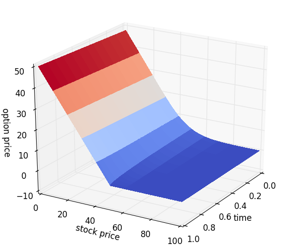
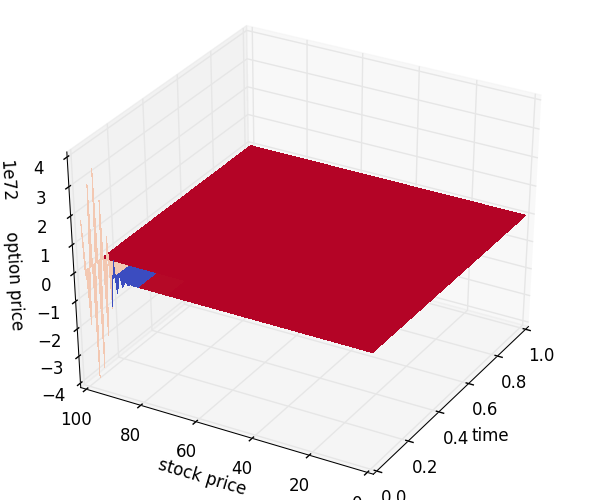
If we set a larger time step, $N=100$, the explicit method might not be stable. As following, we have oscillating option price as our expected.
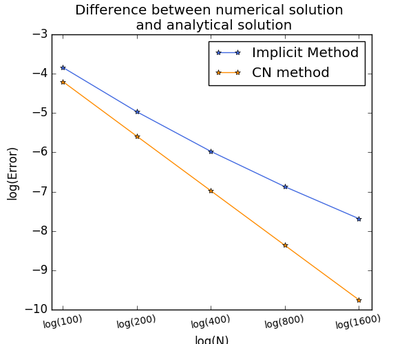
Numerical Convergence
To calculate the error in finite difference method we will take the closed form solution of B-S model for a European put option as the ‘true’ value. Then we compare it the numerical solutions that implicit method and Crank-Nicolson method has produced. As the following plot suggests the numerical solution by implicit method and Crank-Nicolson method converges as $M$ and $N$ increase. We can also find that the Crank-Nicolson method converges fast than the implicit method.