Calibration of Forward Rate Curve
Introduction
Term structure of interest rate describes the relationship between yield and maturity. In practice, the term structure is extensively used by market practitioners to understand conditions in fixed income market and to evaluate various interest rate derivatives. Actually only for several specific maturity the interest rate is known, while the other maturity can be computed by interpolation. To construct the yield curve, many approaches have been proposed. There are parametric methods like Nelson-Siegel model and non-parametric methods such as bootstrapping method and spline methods. The idea of this note is to present all the details of how we have implemented calibration of instantaneous forward rate curve using constrained cubic spline method.
Interest Rate
The time $t$ (today) value of a dollar at time $T \ge t$ is expressed by the zero-coupon bond with maturity $T$ , $P(t, T)$ . Purchasing a zero-coupon bond at $P(t, T)$, holders are guaranteed to be paid one dollar at the maturity $T$ . This leads to the following definitions. Assume $t<S<T$,
The simple forward rate for $[T,S]$ prevailing at t is given by
$$F(t;T,S) = {1\over S-T}({P(t, T)\over P(t, S)}-1) \tag{1}$$
$$\Leftrightarrow 1+(S-T)F(t;T,S)={P(t, T)\over P(t, S)} \tag{2}$$
Through constructing a portfolio, we can deepen our understanding of the simple forward rate. At time t, we sell one unit bond with maturity $T$ and purchase ${P(t, T)\over P(t, S)}$ unit bond with maturity $S$, which means zero net cash flow. Then we have to pay one dollar at time T, while receive ${P(t, T)\over P(t, S)}$ dollars at time S. This is equivalent to that, according to the forward rate for $[T,S]$, we would receive ${P(t, T)\over P(t, S)}$ dollars at time $S$ if invest one dollar at time $T$.The simple spot rate for $[t,T]$ is
$$F(t;t,T) = F(t,T) = {1\over T-t}({1\over P(t, T)}-1) \tag{3}$$
As we know, $P(t,t)=1$ for all $t$The continuously compounded forward rate for $[T,S]$ prevailing at $t$ is
$$f(t;T,S) = -{logP(t,S)-logP(t,T)\over S-T} \tag{4}$$
$$\Leftrightarrow e^{-f(t;T,S)(S-T)}={P(t, T)\over P(t, S)} \tag{5}$$The continuously compounded spot rate, a.k.a. zero rate, for $[t,T]$ is given by
$$f(t;t,T) = z(t,T) = -{logP(t,T)\over T-t} \tag{6}$$
$$\Leftrightarrow P(t,T) = e^{-z(t,T)(T-t)} \tag{7}$$The instantaneous forward rate with maturity $T$ at $t$ is
$$\lim_{S\to T}f(t;T,S) = f(t,T) = -{\partial logP(t,T)\over \partial T} \tag{8}$$$$\Leftrightarrow P(t,T) = e^{-\int_{t}^{T}f(t,u)\mathrm{d}u} \tag{9}$$
Equation $(9)$ reveals the relationship between instantaneous forward rate and zero-coupon bond, in other words, discount rate. Plugging $(9)$ into $(6)$, we have
$$z(t,T) = {\int_{t}^{T}f(t,u)\mathrm{d}u \over T-t \tag{10}}$$
This equation shows that zero rate curve can be built by integrating the instantaneous forward curve.
- The instantaneous short rate at time $t$ is defined by $$\lim_{T\to t}z(t,T) = r(t) = \lim_{T\to t}f(t,T) \tag{11}$$
Related Interest Rate Instruments
- USD 3M LIBOR
- settlement date: 2 business days from the current date
- maturity: 3 months from the settlement date
- convention: following business day convention, end-of-month rule, and ACT/360
- Eurodollar Futures
- underlying instrument: 3-month (90 days) Eurodollar term deposit
- contract expiration date: third Wednesday of each month
- cash settlement to 100 minus ICE 3-month LIBOR
- futures convexity adjustment: A Eurodollar futures buyer would demand higher rate than the corresponding forward contract, resulting a positive convexity adjustment. It can be approximated by $\Delta(t_1,t_2) = L_{fut}(t_1,t_2) - L_{fwd}(t_1,t_2)\approx {1\over 2}\sigma^2t_1t_2$
- Interest Rate Swap (payer interest rate swap)
- notional value: N
- fixed rate: K
- a series of futures dates $T_{0} < T_{1} < T_{2} < ...< T_{2n}$ with $T_{i}-T_{i-1}=0.25$ (in years). $T_{0}$ is 2 business days from t.
- The payer pays fixed rate K on $T_{2i}$ for the period $[T_{2i-2},T_{2i}]$
- The payer receives payment on $T_{i}$ for the period $[T_{i-1},T_{i}]$ according to 3-month LIBOR rate
- convention: following business day convention, end-of-month rule, and ACT/360
Cubic Spline Interpolation Methodology
Interpolation is a method of estimating the value of a function using the known data points. As global interpolation is subject to oscillation and overshoot problem, we prefer to use piecewise interpolation method. Linear interpolation rely on concatenating linear polynomial between each pair of data points. Although it never overshoots or oscillates, it result in a discontinuous derivative. Consider the trade-off between smoothness and overshooting, here we prefer the cubic spline method.
For traditional cubic spline, we need to construct $N$ third degree polynomial $f_{i}(x)$ , with coefficients $a_{i}$, $b_{i}$, $c_{i}$, $d_{i}$ , for each pair of points $[x_{i}, x_{i+1}], 0\leq i\leq N-1$
$$f_{i}(x) = a_{i} + b_{i}x + c_{i}x^2 + d_{i}x^3 \tag{12}$$
Cubic spline function $f_{i}(x)$ is constructed based on the following criteria:
$$f_i(x_i) = y_i \tag{13}$$
$$f_{i+1}(x_i) = y_i \tag{14}$$
$$f_i^{'}(x_i) = f_{i+1}^{'}(x_i) \tag{15}$$
$$f_i^{''}(x_i) = f_{i+1}^{''}(x_i) \tag{16}$$
$4N$ coefficients need to be solved, but we only have $4N-2$ coefficients. Extra conditions are needed to solved the equation set.
For interest rate curves, constraint spline is a good choice to avoid overshooting. Most importantly, specifying first order derivative replaces the requirement for equal second order derivative at each point. So we have
$$f_i^{'}(x_i) = f_{i+1}^{'}(x_i) = f^{'}(x_i) \tag{17}$$
Specifically, the first derivative of each point is the harmonic average of the slopes of the adjacent straight lines, and should equal to zero if the slope change sign at point.
$$f^{'}(x_i)= {2 \over {x_{i+1}-x_{i}\over y_{i+1}-y_{i}} + {x_{i}-x_{i-1}\over y_{i}-y_{i-1}}} $$
$$= 0\ if\ slope\ changes\ sign\ at\ point$$
As slope of each point is known, we can directly calculate each spline function instead of solving a system of equations.
$$d_i = {f_{i}^{''}(x_i)-f_{i}^{''}(x_{i-1})\over 6(x_i-x_{i-1})}$$
$$c_i = {x_{i}f_{i}^{''}(x_{i-1})-x_{i-1}f_{i}^{''}(x_{i})\over 2(x_i-x_{i-1})}$$
$$b_i = {(y_i-y_{i-1}) - c_i(x_i^2-x_{i-1}^2) - d_i(x_i^3-x_{i-1}^3)\over (x_i-x_{i-1})}$$
$$a_i = y_{i-1} - b_ix_{i-1} - c_ix_{i-1}^2 - d_ix_{i-1}^3$$
Interest Rate Curve Fitting
In practice, we only observe the market quotes of interest rate instruments instead of points on the forward rate curve. To obtain the forward curve, we need to calibrate an instantaneous forward rate curve to fit the market quotes. Following are the steps of algorithm construction,
- Compute the times of nodes which used as known points for interpolation
- Assume the initial forward rate at node $S_i$ is $y_i$. Construct constrained cubic spline for each pair of nodes
- Derive the times and amounts of the cash flow for each instrument. Here are 3 examples to illustrate the details.
- USD 3M LIBOR: This case is straightforward. The first cash flow is $-1$. The second one is $1+{r\over 100}{30\over 360}$
- Eurodollar futures contract: There are two cash flows. The first one is $1-F/4$ which happens at the settlement $t$. The second one is $1$ happens at $t+0.25$. $F$, the forward rate, can be calculated using this equation $F = 1 - Q/100 - 0.5\sigma^2t(t+0.25)$. $1-Q/100$ is the futures rate and $Q$(out of $100) is the futures quote.
- 2-year Swap with fixed coupon c: There are five cash flows: $-1$ at time 2 business days from today, $c/2$ at the end of each $6$ month after $2$ business days, $1+c/2$ at $2$ B-days + $24$ months
- Calibrate the forward rate $y_i$ at node $S_i$ by making the NPV of instrument i to 0 successively.
- write a function which takes argument $y_i$ and calculates the integral of forward rate curve between each given cash flow times $t_{j}$ and origin. Hence, discount factors can be calculated using $P(t,T) = e^{-\int_{t}^{T}f(t,u)\mathrm{d}u}$
- write a function which takes argument $y_i$ and calculates the NPV of instrument i: $NPV(y_i) = A_{i1}P_{i1}(y_i) + A_{i2}P_{i2}(y_i) + ... +A_{in}P_{in}(y_i)$ . $n$ is the number of cash flows for instrument $i$.
- Use Scipy function fsolve to solve for $y_i$ such that $NPV(y_i) = 0$ and replace the old $y_i$ with the new one
- Stopping rule
- the maximum number of calibration is exceeded.
- the maximum change of forward rates is less than a threshold.
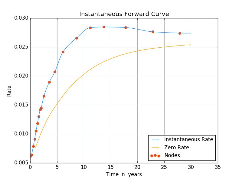
Numerical Results
In summary, we have constructed the instantaneous forward rate curve from several instruments including USD 3M LIBOR, Eurodollar futures, and Swaps. The blue curve is the instantaneous forward curve and the yellow curve is the zero rate curve, which is constructed by integrating the forward curve.